Electrical Resistivity Tomography (ERT)
Need and Scope:
Understanding subsurface conditions is critical for geotechnical, civil, and environmental engineering applications. Conventional invasive methods, such as drilling or coring, provide reliable but localized information, often at high cost and with disturbance to the structure. Electrical Resistivity Tomography (ERT) offers a non-destructive alternative that enables continuous imaging of the subsurface. It is particularly useful for identifying stratigraphy, detecting anomalies such as voids or weak zones, evaluating material uniformity, Groundwater detection, and monitoring changes over time. The technique allows flexible deployment in 1D, 2D, and 3D configurations depending on project requirements.
Concept:
ERT methodology involves injecting a direct current between two surface current electrodes(AB) while two additional electrodes (MN) gauge the voltage drop. Deeper depths can be explored by adjusting or increasing the spacing and layout of the electrodes. When conducting an ERT survey, electrodes are arranged in a specific configuration on the ground, tailored to the desired depth and anticipated subsurface structure. Typical setups include Schlumberger, Wenner, and Dipole-Dipole, Pole-Pole, Pole-Dipole, and Gradient arrays. Following electrode placement, the resistivity meter applies current between two current electrodes, with the potential difference measured between two other potential electrodes. This procedure is repeated for differing electrode spacings to gather data at different depths. Subsequently, the collected data is analyzed to ascertain resistivity values at varying depths. The calculated resistivity value is an apparent value, or the resistivity of a homogeneous ground, that will produce the same resistance value for the same electrode setup, rather than the actual resistivity of the subsurface. The connection between the apparent and the true resistivity is complicated. Therefore, the inversion problem uses the apparent resistivity readings to calculate the true subsurface resistivity.
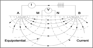
Fig 1. Current flow path for the four-electrode system
For a four-point electrode system, the voltage difference between the potential electrodes is given by
where VMN is the voltage between the two potential electrodes, ρ is the apparent electricity obtained, and I is the Electric current applied. rAM = rMB = rAN = rBN is the distance between the respective current and potential electrodes. This equation is used to compute potential distribution under the subsurface and Apparent resistivity using geometric factors.
Electrical Resistivity Tomography (ERT)
Test Setup and Accessories:
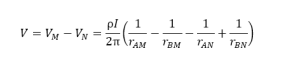
The equipment used for testing is the AIMIL stacked Deep Resistivity meter 125W-400V-2A. This Resistivity Meter is a single-unit integrated device comprising a transmitter and a receiver, and it comprises
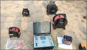
Fig 2. ERT Instrument
- Two voltage meters
- Two Current meters
- External Battery
- Connecting cables
- Steel rod electrodes
- Display System
Before conducting the survey, the following array configuration details should be selected based on the type of array used for the survey and the depth of investigation.
- Type of array used
- Total Survey Length (L)
- Initial Spacing between the electrodes (a)
- Total No of Data Levels(n)
- Total No of Data points in the 2D survey (N2d)
- Total No of Data points in the 1D survey (N1d)
- Depth of Investigation Covered (Ze)
Fig 3. Sample 2D Data Configuration layout of a Survey
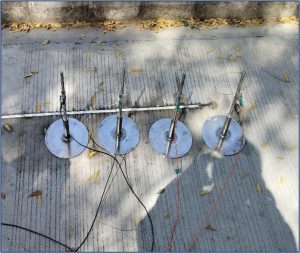
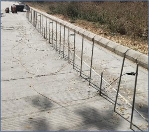
Fig 4. ERT Testing in Pavements: a) using circular steel plates placed in pavement, b) using steel rod electrodes placed in drilled holes
Electrical Resistivity Tomography (ERT)
Following data acquisition, the raw data is processed through structured input preparation, removal of outliers, if any, and application of smoothing and noise filtering if needed. The refined dataset should be analyzed using a two-stage framework: (i) forward modeling to simulate resistivity responses, and (ii) inversion modeling to estimate the true subsurface resistivity distribution.
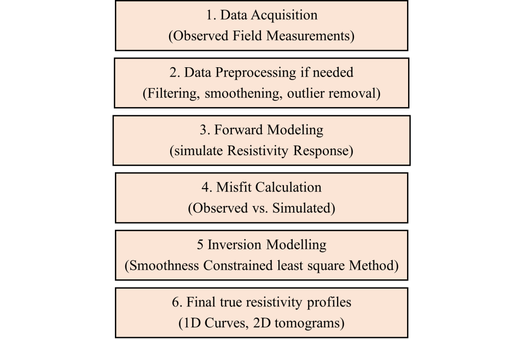
Fig 5. Flowchart for Data Analysis
While 1D inversion provides vertical resistivity variation with depth, 2D inversion offers tomographic visualization across both depth and horizontal extent, enabling reliable interpretation of pavement layers and subsurface conditions. The two-stage framework can be analyzed using RES2DINV or other commercial software or custom codes.
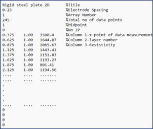
Fig 6. Sample input file format for the 2D Data
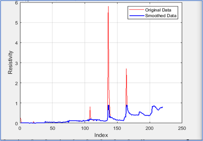
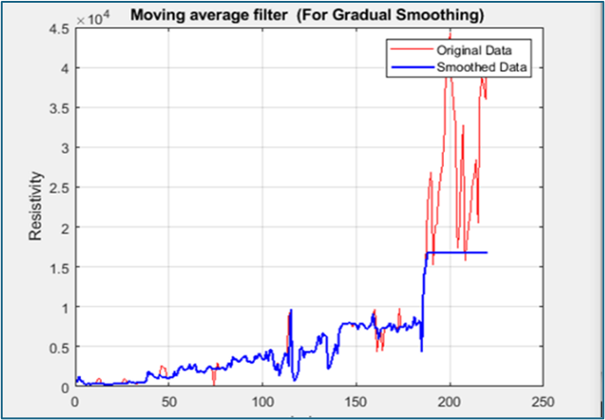
Fig 7. Hampel Filtering and IQR for removing noise
- Always compare before and after filtering plots.
- Never filter the data without interpreting outliers in a geological/geotechnical context.
- If unsure about an anomaly, repeat measurements at that location to confirm.
- When using custom codes for post-processing, it is essential to incorporate the role of convergence parameters. Key factors such as the regularization parameter, weighting components, mesh size, and iteration stabilization parameters must be carefully considered. Defining the appropriate ranges for these parameters is critical to ensure stable and reliable inversion results.
Electrical Resistivity Tomography (ERT)
The results presented here demonstrate the determination of pavement layer thickness in both rigid and flexible pavements using the custom code ERTPAVE. The locations of the ERT measurement points are indicated by black dots in the measured and calculated pseudo-section plots.
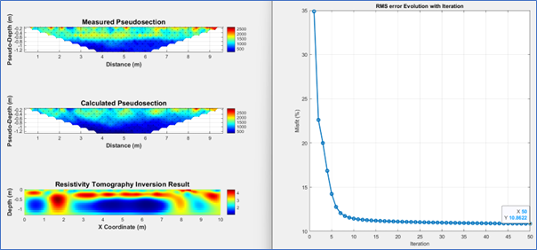
Fig 8 2D Fine Mesh – Rigid Pavement
The following observations are made for the thickness interpretation of Rigid Pavement from Fig. 8,
- Concrete slab extends to ~0.3 m depth (cyan–yellow zone).
- High-resistivity granular subbase observed between 0.3–0.5 m (red zone).
- Uniform low-resistivity subgrade soil present below 0.5 m.
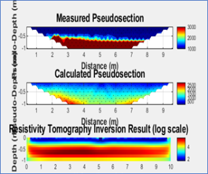
Fig 9 2D Fine Mesh – flexible Pavement
The following observations are made for the thickness interpretation of Flexible Pavement from Fig. 9.
- Initial blue region indicates the presence of WBM having a thickness of about 0.2m
- Granular subbase layer (cyan region) varies from 0.2m to 0.4m in depth.
- The rest is subgrade soil after 400mm.
Limitations of ERT Survey:
- It can be challenging to place the electrodes on surfaces like bare rock or extremely hard, dry, or frozen ground. Drilling may be necessary. Custom plate electrodes could be an option in some situations.
- Other geophysical techniques are advised for investigations deeper than 500 meters.
- Closely spaced electrodes are necessary to achieve high-resolution data, which lengthens fieldwork.
Electrical Resistivity Tomography (ERT)
Theory:
Electrical Resistivity Tomography (ERT) is based on the principle that different subsurface materials exhibit different electrical resistivity. When an electrical current is injected into the ground through a pair of electrodes, the potential difference is measured at other electrode pairs. Using Ohm’s law, these measurements are converted into apparent resistivity values, which reflect the bulk response of the subsurface. The relationship between current flow, electric field, and resistivity is governed by the continuity equation and Ohm’s law in differential form. The forward problem in ERT involves computing the potential distribution for a given resistivity model, whereas the inverse problem estimates the true resistivity distribution from field measurements. Since inversion is an ill-posed problem, regularization techniques such as smoothness constraints are applied to stabilize the solution and avoid unrealistic fluctuations. Different electrode configurations (e.g., Wenner, Schlumberger, Dipole–Dipole) control the resolution and depth of investigation. The Shallow, high-resolution imaging can be achieved with closely spaced electrodes, while deeper layers require wider spacing. The final inversion output is usually presented as 1D profiles or 2D/3D tomographic images, which can be interpreted in terms of soil stratigraphy, groundwater levels, rock properties, or structural defects.
References:
- Dey, A., & Morrison, H. F. (1979). Resistivity modeling for arbitrarily shaped three-dimensional structures. In GEOPHYSICS (Vol. 4, Issue 3).
- Mark E. Everett (2013). Near Surface Geophysics. Cambridge University Press (Book)
- Spitzer, K. (1998). The three-dimensional DC sensitivity for surface and subsurface sources. Geophysical Journal International, 134(3), 736–746