Strain Localization
Need and Scope:
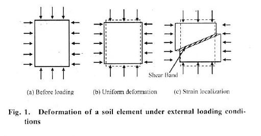
When a uniformly homogeneous material is subjected to low homogeneous loading, homogeneous deformations occur. As deformations become larger, concentration of strain at local zones is observed throughout the height of the sample. Failure of specimen is characterized by formation and propagation of these localized deformations. Strain localization is considered a major factor that governs the mechanical response of a specimen, at or near failure.
(Sachan and Penumadu 2007)
Concept:
Failure of many engineering material is characterized by the formation and propagation of zones of localized shear deformation. Strain localization is caused by the imperfections inherent in the soil specimen, boundary constraints and non-uniform loading conditions. The most typical localized deformation observed in geo-material is linear shear banding. Shear band is a narrow zone of intense straining and is one of the possible deformation modes precursor to catastrophic failure.
Strain Localization
Experimental Setup:
- Triaxial loading frame
- Load cell
- LVDT
- Triaxial cell
- Soil specimen
- DAQ & computer system
- Cell Pressure control
- Pore Pressure control
- Volume change device
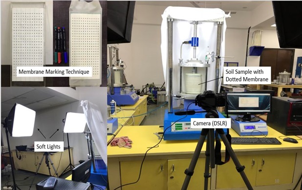
- Latex membrane with dot markings
- DSLR camera
- Soft lights
- Camera Tripod
Testing procedure:
In a normal CU/CD triaxial test, following things need to be done in order to obtain strain localization patterns. The procedure for performing CU test can be referred from https://research.iitgn.ac.in/stl/cutriaxial.php#
- The latex membrane of thickness 0.3mm with dots marked in a grid pattern should be used. Grid points are spaced approximately 10mm apart.
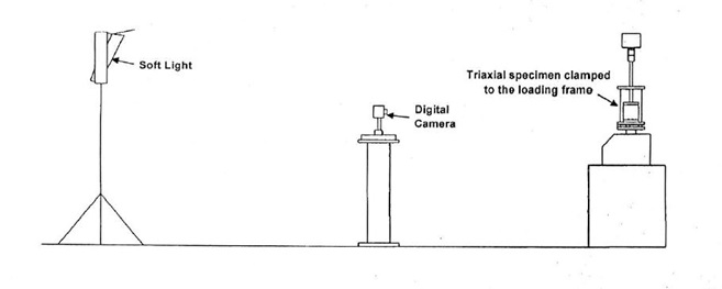
- The dots on the specimen (latex membrane) are tracked using high-resolution digital images. To obtain digital images of triaxial specimen, a DSLR camera is placed at a distance of 562mm from the outer wall of cell.
- The DSLR camera is mounted on a two-axis controller tripod, which allows for precisely adjusting camera position in two directions. Camera focus is manually adjusted using zoom and direction controller in order to have the specimen placed vertically in the center of the image.
- Soft lights are used in order to have high quality images, which would help in tracking dots more precisely using software. Soft lights are placed in such a manner that illumination on sample is maximum with no glaring effect observed from triaxial cell.
- Digital images of specimen are taken during shearing stage. Timer is set in camera in order to have images captured of specimen at different intervals of time. While Images are being captured, no disturbance should be given to the camera. The interval of each image can be set in accordance to requirement of strain contour in respect to global strain level.
- Digital images of specimen after shearing is complete are downloaded onto a personal computer so that they can be processed using software.
Strain Localization
Experimental Setup:
Digital images of specimen captured during shearing are processed using Geo-PIV matlab module. (Stanier et.al 2015)
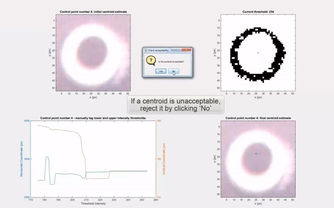
- Coordinate of marked points on specimen lying under plane of interest are determined using geopiv matlab module. One has to create a control point file in matlab, in order for geopiv module to help find the coordinate of all the nodes (plane of interest). The user with the help of geopiv matlab module does the centroiding of each node manually using threshold intensity. Coordinates of all the nodes for all the images are found using this procedure.
- Once, the coordinate of nodes are determined by the user for all digital images one can correct them for refraction correction. In triaxial testing, the refraction of light will cause the specimen to appear enlarged. Therefore, correction must be applied to the data obtained from digital images in order to determine true specimen dimensions and grid point positions. By incorporating Snell’s Law of refraction, a 2D correction model (Parker 1987; Lin and Penumadu 2005) is used.
- After applying refraction correction, the coordinates of all nodes in different images are again fed back to geopiv matlab module, which in turn helps us to find strain.
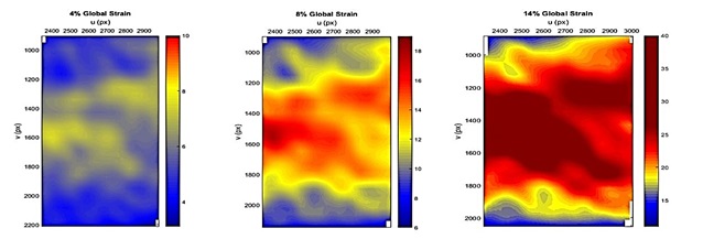
- Strain contours of specimen at different global strain levels are plotted using the geopiv matlab module. These strain contours can be found in respect to the absolute strain (with reference to image taken at zero strain level) or can be found in respect to incremental strain depending upon the requirement.
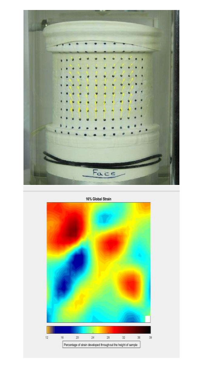
Finding target point coordinates using Geopiv-rg
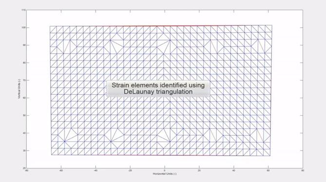
Calculation of strain elements using Geopiv-rg
Plotting of Strain contours
Strain Localization
Example:
A triaxial test was performed on a cohesive soil. The in-situ density and in-situ water content of soil was 1.9 gm/cc and 20% respectively. The strain controlled triaxial test was performed on a specimen at a deformation rate of 0.5mm per minute. The size of the specimen was 100 mm in diameter and 200 mm in height.�
General Remarks:
- Camera should be kept undisturbed during shearing stage and should be properly aligned in direction of sample. Battery should be fully charged so that it would last the entire period of testing. If the deformation rate is very slow then external power source should be used for the camera.
- The timer in camera should be synced with respect to global strain level in order to have image of specimen at that global strain level. It will help to know at what global strain level, strain localization initiated and how it will progress.
- The soft light should provide sufficient illumination in order to remove all the shades of darkness from the region of interest.
Strain Localization
Theory:
To address the strain localization and its impact on the interpretation of test results, the deformation and strain components at various locations of a deforming specimen are needed. However, direct measurement of deformation at various locations along the height of the specimen is a difficult experimental task. Digital image analysis is a technique that helps to evaluate the strain localization occuring on a soil specimen when sheared. Images of the specimen at various intervals of time during shearing stage are taken and the particles or target points are tracked in various images to compute their new coordinate. With the help of new coordinate of tracked target points user can evaluate the localized deformation that is occurring throughout the height of the sample. The target points are identified using centroid of the intensity peak created by a colored target on a contrasting background.
(White 2003, Stanier et.al 2015)
References
- Sachan, A., & Penumadu, D. (2007). Strain localization in solid cylindrical clay specimens using digital image analysis (DIA) technique. Soils and foundations, 47(1), 67-78.
- Stanier, S. A., Blaber, J., Take, W. A., & White, D. J. (2015). Improved image-based deformation measurement for geotechnical applications. Canadian Geotechnical Journal, 53(5), 727-739.
- White, D. J., Take, W. A., & Bolton, M. D. (2003). Soil deformation measurement using particle image velocimetry (PIV) and photogrammetry. Geotechnique, 53(7), 619-631.